x = 1; x = x+input()if(x < 0) { x = -1 * x}
|
input represents some value entered by a user |
 |
What is the value of x here? |
This is a recap of the paper "Abstract Interpretation" written by by Patric Cousout released 1996 by ACM. You can find it here: doi.org/10.1145/234528.234740
I am in no way knowledgeable. This is only a recap, expect errors!
The Semantic of a program is the meaning of a program. The semantic is written in an programming language. A programming language has a syntax which defines which combinations of characters describe valid programs and which aren’t. It’s important to distinguish between syntax and semantic. A semantic describes the steps a computer is doing to evaluating program based on rules. This rules are written down in a semantic domain called \(D\).
For small-step operational semantics \(D\) can be a transition systems and for big-step operational semantics \(D\) can be a pom-set or trace-relations.

|
More about semantic
Semantics in General: en.wikipedia.org/wiki/Semantics_(computer_science)
|
Assume we’ve got a program \(p\) with a concrete Semantic \(S\). We are interested in some properties of this program. For example the value of a variable in this program:
x = 1; x = x+input()
|
input represents some value entered by a user |
|
What is the value of x here? |
We cannot conclude the exact value of x is at point 2, but if we are, e.g. only interested in the sign of \(x\) we are able to provide an answer. This process is called abstraction of the Domain and to assert properties of a program within this abstract domain is called "Abstract interpretation"
Patrick Cousot introduces Abstract interpretation as the general theory to approximating the semantics of a discrete dynamic system. A program written in a imperative programming language can be such a system. There is a state representing all variables and assignments changing that state for concrete variables.
The Semantics of a program \(p\) written in a programming language \(L\) is represented as a value \(S \llbracket p \rrbracket \in D \).
\(D\) represents a semantic domain. Examples of such domains can be found in section Semantics
The first step towards abstract interpretation of a program \(p\) written in a language \(L\) and in the domain \(D\) is to abstract the domain to an abstract domain \(D^\#\) that only consist of properties we want to have an assertion on. E.g.: \(Values(x) \supe signs(x)\).
If we draw a Ven-diagramm of the above it would look like:
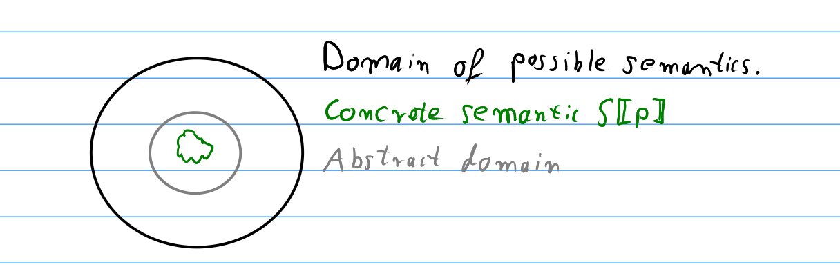
For this abstract domain we choose an abstract Semantics \(S^\# \in L \mapsto D^\#\). The abstract Semantics is usually intuitively defined for \(L\).
As next step a "soundness-relation" that maps a Semantic to a corresponding abstract Semantic is proven that is holds:
Now we can assure that our abstract semantics can represent any semantic that is possible to compute in the language \(L\). This proof can be costly because usually this can’t be automated.
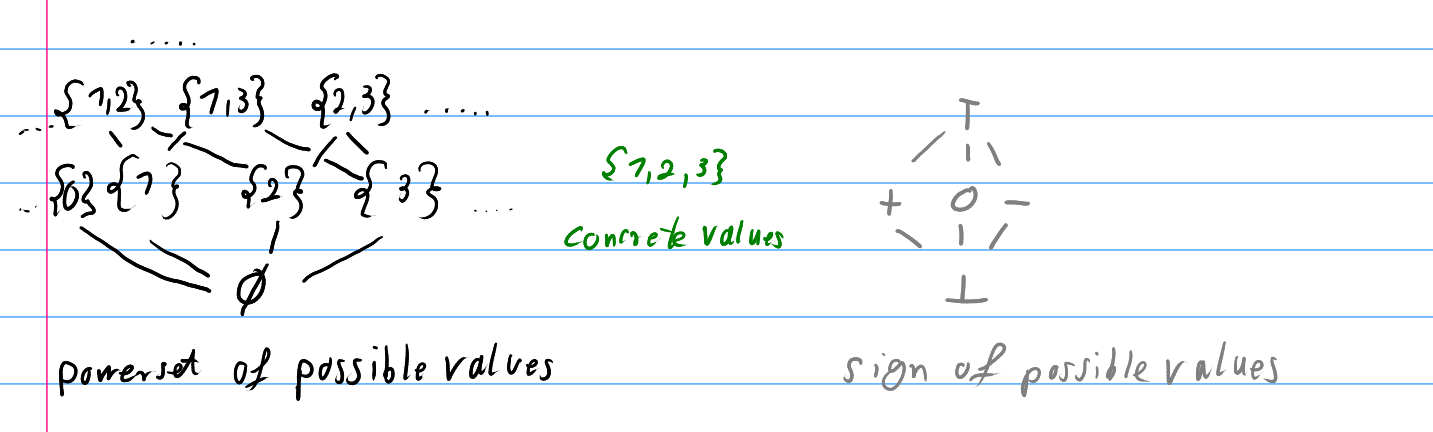
Cousot introduced a different approach. The state of a program is represented as powerset of all variables and their possible values. This powerset is the domain \(D\) of the program \(p\) and the semantic function \(S\llbracket p \rrbracket\) maps a given program to his state.
Then, just as in the Empirical approach, an abstract domain \(D^\#\) is chosen which only represents the properties we are interested in. \(D^\#\) should be a powerset-lattice with the properties for all variables we want to monitor. Now we can define a semantics \(S_{coll} \llbracket p \rrbracket \in L \mapsto D^\#\). Concrete \(S^\#\) is an abstract representation of all possible values of the concrete semantics. Cousot proves that \(S_{coll} \llbracket p \rrbracket\) is the best approximating of the semantics / behaviour of our program \(p\).
A example for this for the abstraction of the "sign" of values would look like this:
The abstraction function \(\alpha\) maps concrete object \(o\) to abstract objects \(o^\#\), it "simplifies" \(o\).
The concretization function \(\gamma\) maps an abstract object \(o^\#\) to the largest concrete object \(o\).
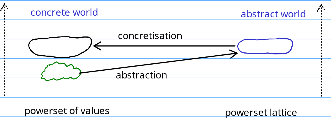
\(\gamma(d): \: D^\# \mapsto D\) |
\(\alpha(S): \: D \mapsto D^\#\) |
\(D\) is the poweset of values |
\(D^\#\) is the sign lattice \(\{ \top, \bot, +, -, 0 \}\) |
After choosing \(D^\#\) we need to define the abstract semantics function \(S^\# \llbracket p \rrbracket\). It convenient to do so via induction on the structure of the program \(p\).
\(S^\# \llbracket x:= r \rrbracket = sign(r)\) where \(r \in \mathbb{R}\).
\(S^\# \llbracket x:= y \rrbracket = S^\# \llbracket y \rrbracket \) where \(y\) is a variable.
\(S^\# \llbracket x:= z + y \rrbracket = S^\# \llbracket z \rrbracket +_a S^\# \llbracket y \rrbracket \) where \(y, z\) are variables.
One disadvantage of this definition is that in general our abstract semantics function is only a superset of the best approximation that would be possible. Our soundness proof follows due to the inductive definition. Therefore we save quite a bit of work here compared to the Empirical approach
A Galois connection is a tuple of 2 functions \((\alpha, \gamma)\). In our case the abstraction function \(\alpha\) and the concretization function \(\gamma\). Formally our Galois is defined as two sets:
\(D(\sube, \cap, \emptyset, Z^d)\) and \(D^\#(\sqsubseteq^\#, \sqcap^\#, \bot, \top)\)
and the function tuple:
\((\alpha = D \mapsto D^\#, \gamma = D^\# \mapsto D)\)
where \(\forall x \in D. \: x \sube \gamma ( \alpha (x))\).
Our connection \((\alpha, \gamma)\) is called a Upper-adjointment if:
\( \forall x, y \in D. \: \alpha(x) \leq y \iff x \leq \gamma(y)\)
We choose our approximation function \(\alpha\) as a upper-adjointment of a Galois connection. Therefore we can assure it exists and is the best possible approximation.
Abstract interpretation can be used to:
Proof a program is free of certain errors.
Check if a compiler can apply certain optimizations in a secure way.
Generate test-inputs for programs for debugging.
Type interference during compilation
